반응형
1. 스칼라와벡터
1.1 벡터그리기
import math
import matplotlib.pyplot as plt
import numpy as np

a = [6,13]
b = [17,8]

plt.figure(figsize=(10,10))
plt.xlim(0, 20)
plt.ylim(0, 20)
plt.xticks(ticks=np.arange(0, 20, step=1))
plt.yticks(ticks=np.arange(0, 20, step=1))

plt.arrow(0, 0, a[0], a[1], head_width = .5, head_length = .5, color = 'red')
plt.arrow(0, 0, b[0], b[1], head_width = .5, head_length = .5, color = 'blue')


plt.axhline(0, color='gray', alpha = 0.3)
plt.axvline(0, color='gray', alpha = 0.3)
plt.title("Vector")
plt.grid()
plt.show()
1.2 a⃗ −b⃗ 그리기
a = [6,13]
b = [8,8]
c = [a[0]-b[0],a[1]-b[1]]
plt.figure(figsize=(10,10))
plt.xlim(-10, 15)
plt.ylim(-10, 15)
plt.xticks(ticks=np.arange(-10, 15, step=1))
plt.yticks(ticks=np.arange(-10, 15, step=1))

plt.arrow(0, 0, a[0], a[1], head_width = .5, head_length = .5, color = 'red')
plt.arrow(a[0], a[1], -b[0], -b[1], head_width = .5, head_length = .5, color = 'green')
plt.arrow(0, 0, c[0], c[1], head_width = .5, head_length = .5, color = 'blue')

plt.axhline(0, color='gray', alpha = 0.3)
plt.axvline(0, color='gray', alpha = 0.3)
plt.title("Vector")
plt.grid()
plt.show()
1.3 a⃗ 와 스칼라의 곱
a = [8,12]
five = np.multiply(5, a)
minus_three = np.multiply(-3, a)

plt.figure(figsize=(10,10))
plt.xlim(-40, 65)
plt.ylim(-40, 65)
plt.xticks(ticks=np.arange(-40, 65, step=5))
plt.yticks(ticks=np.arange(-40, 65, step=5))

plt.arrow(0, 0, a[0], a[1], head_width = 2, head_length = 3, color = 'red', alpha=0.7)
plt.arrow(0, 0, five[0], five[1], head_width = 2, head_length = 3, color = 'blue', alpha=0.3)
plt.arrow(0, 0, minus_three[0], minus_three[1],width=0.6, head_width = 2, head_length = 3, color = 'green', alpha=0.2)

plt.axhline(0, color='k')
plt.axvline(0, color='k')

plt.title("Vector")
plt.grid()
plt.show()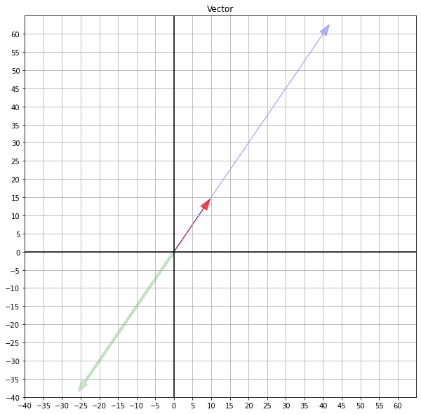
1.3 3D vector
from mpl_toolkits.mplot3d import Axes3D

vectors = np.array([1,0,0,0,1,0,0,0,1]).reshape(3,3)
X, Y, Z = zip(*vectors)
fig = plt.figure()
ax = fig.add_subplot(projection='3d')
ax.quiver(0,0,0,X, Y, Z, length=1)
ax.set_xlim([-1, 1])
ax.set_ylim([-1, 1])
ax.set_zlim([-1, 1])
ax.set_xlabel('X')
ax.set_ylabel('Y')
ax.set_zlabel('Z')
plt.show()
1.4c⋅d (Dot Product)
c = [6,4,17,18]
d = [7,8,21,6]
f = [v*w for v,w in zip(c,d)]
f = np.sum(f)
print(f) # 곱한 뒤 sum으로만계산
print(np.array(c).dot(np.array(d))) #numpy사용
539
539
1.5 e x f (행렬곱)
e = np.array([7,21,10]).reshape((3,1))
f = np.array([8,1,5]).reshape((1,3))
print('e\n',e)
print('f\n',f)
print('e X f\n',np.matmul(e,f))
print('e . f\n',np.dot(e,f))
# 행렬곱에서 dot을 해도 값이 똑같이 나온다.
# 이는 프로세스가 거의 비슷해서인데, 2차원까지는 거의 같다고 봐도 무방.
# 하지만 고차원으로 가면 달라지는데 이는 Tensorflow등을 이용하므로 skip
1.8 ||a|| 와 ||b|| 계산 (NORM)
from numpy import linalg as LA
a = np.array([-7,9,5,-10]).reshape((4,1))
b = np.array([1,1,-8,17]).reshape((4,1))
print('norm of vector g :',LA.norm(a))
print('norm of vector h :',LA.norm(b))
def get_norm (a):
  s = np.square(a).sum()
  return np.sqrt(s)
print(get_norm(a))
2. 매트릭스
2.1 FT를 계산
F = np.array([3,65,3,35,25,8,0,0,3,4,96,72]).reshape((4,3))
print(F)
print(F.T)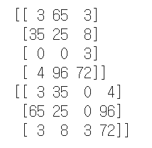
2.2 IA 를 계산
from numpy import linalg as LA
A = np.array([6,1,0,3]).reshape(2,2)
I = np.identity(A.ndim)
print(np.identity(2))
print(I)
print(I.dot(A))
2.3 I 구하기
from numpy import linalg as LA
A = np.array([-17,11,10,3]).reshape(2,2) # A
A_inv = LA.inv(A) # A -
unit = A.dot(A_inv) # A A-
A.dot(unit) # A I

unit.dot(A) # I A

print(unit.dot(A))
print(unit) # 컴퓨터로 계산하는 것이기 때문에 1과 0에 '근사한'수치가 나옴
print(unit.astype(int))
H = np.array([8,18,-4,12]).reshape(2,2)
H_inv = LA.inv(H)
J = np.array([-10,6,-6,2,3,-2,3,-1,-8]).reshape(3,3)
J_inv = LA.inv(J)

print(H.dot(H_inv))
print(J.dot(J_inv).round())
2.4 |A| 와 |B|를 계산 (Determinant)
from numpy import linalg as LA
A = np.array([8,18,-4,12]).reshape(2,2)
BlockingIOError = np.array([-10,6,-6,2,3,-2,3,-1,-8]).reshape(3,3)
print('|A| :',LA.det(A))
print('|B| :',LA.det(B))
2.5 H−1 와 J−1 를 계산 (Inverse)
from numpy import linalg as LA
print('inverse of A :\n',LA.inv(A))
print('\ninverse of B :\n',LA.inv(B))
2.6 행렬 코드만들기
x = np.array([1,0]); y = np.array([0,1])
mat = np.array([x, y])
det_mat = np.linalg.det(mat)
print('Matrix: \n' , mat)
print('det:', det_mat)
print('-'*40)
#rotate mat 90 dgree
rot_90 = rot = np.array([[np.cos(deg), -np.sin(deg)], [np.sin(deg), np.cos(deg)]])
mat_rotated = np.matmul(mat, rot_90).round(2)
print('Rotated Matrix: \n' , mat_rotated)
print('det:', np.linalg.det(mat_rotated))
print('-'*40) # Here we can see the rotation of the matrix doesn't affect the area

print('Stretched Matrix: \n' , np.array([2*x, y]))
print('det:', np.linalg.det(np.array([2*x, y])))
print('-'*40) # Here we can see the strech of the matrix 2 times bigger area than the original

print('Stretched Matrix: \n' , np.array([x, 2 * y]))
print('det:', np.linalg.det(np.array([x, 2 * y])))
print('-'*40) # Here we can see the strech of the matrix 2 times bigger area than the original

print('Stretched Matrix: \n' , 2*np.matmul(mat, rot_90).round(2))
print('det:', np.linalg.det(2*np.matmul(mat, rot_90).round(2)))
print('-'*40) # Here we can see the strech of the matrix 4 times bigger area than the original

print('Rotated and Stretched Matrix: \n' , 2 * mat_rotated)
print('det:', np.linalg.det(2 * mat_rotated))
print('-'*40) # Here we can see the strech of the matrix 4 times bigger area than the original
반응형
'기본소양 > 선형대수학' 카테고리의 다른 글
| 파이썬으로 하는 선형대수학 (4. 공분산과 상관계수) (0) | 2021.01.18 |
|---|---|
| 파이썬으로 하는 선형대수학 (3. Span, Rank, Basis, Projection) (0) | 2021.01.18 |
| [선형대수학] 차원을 왜 축소시키는가 (0) | 2021.01.15 |
| [선형대수학] 공분산과 상관계수 ( 피어슨, 스피어만) (0) | 2021.01.14 |
| [선형대수학] 고유값과 고유벡터, 벡터의 변환 (0) | 2021.01.14 |


댓글